GPU Isosurface Polygonalization

Posted by andrewgotow on August 21, 2018

Isosurfaces are extremely useful when it comes to data visualization. From medical imaging to fluid flow analysis, they are an excellent tool for understanding complex volumetric data. Games have also adopted some of these techniques for their on purposes From the more rigid implementation in the ubiquitous game Minecraft to the Gels in Portal 2, these techniques serve the same basic purpose.

I wanted to try my hand at a general-purpose implementation, but before we dive into things, we must first answer a few basic questions.

What is an isosurface?

An isosurface can be thought of as the solution of a continuous function which produces a constant output in 3D. If you’re visualizing an electromagnetic field for example, you might generate an isosurface for a given potential, so you can easily determine its overall shape. This technique can be applied to other arbitrary values as well. Given CT scan data, a radiologist could construct an isosurface at the density of a specific type of tissue, extracting a 3D representation of bones or organs to view them separately, rather than having to manipulate a less intuitive stack of images.

What will we use this system for?

I don’t work in the medical field, nor would I trust the accuracy of my implementation when it comes to making a diagnosis. I work in entertainment and computer graphics, and as you would imagine, the requirements are quite different. Digital artists can already craft far better visuals than any procedure yet known; the real challenge is dynamic data. Physically simulated fluids, player-modifiable terrain, mechanics such as these present a significant challenge for traditional artists! What we really need is a generalized system for extracting and rendering isosurfaces in real time to fill in the gaps.

What are the requirements for such a system?

Given our previous use case, we can derive a few basic requirements. In no particular order…

The system must be intuitive. Designers have other things to do besides tweaking simulation volumes and fiddling with configurations.
The system must be flexible. If someone suggests a new mechanic which relies heavily on procedural geometry, it should be easy to get up and running.
The system must be compatible. The latest experimental extensions are fun, but if you want to release something that anyone can enjoy, it needs to run on 5 year old hardware.
The system must be fast. At 60 fps, you only have 16ms to render everything in your game. We can’t spend 10 of that drawing a special effect.

Getting Started!

Let’s look at requirement no. 4 first. Like many problems in computing, surface polygonalization can be broken down into repeated instances of much smaller problems. At the end of the day, the desired output is a series of interconnected polygons which appear to make up a complex surface. If each of these component polygons is accounted for separately, we can dramatically reduce the scope of the problem. Instead of generating a polygonal surface, we are now generating a single polygon, which is a much less daunting task. As with any discretization process, it is necessary to define a regular sample interval at which our continuous function will be evaluated. In the simplest 3D case, this will take the form of a regular grid of cells, and each of these cells will form a single polygon. Suddenly, this polygonalization process becomes massively parallel. With this new outlook, the problem becomes a perfect fit for standard graphics hardware!

For compatibility, I chose to implement this functionality in the Geometry Shader stage of the rendering pipeline, as it allows for the creation of arbitrary geometry given some basic input data. A Compute Shader would almost definitely be a better option in terms of performance and maintainability, but my primary development system is OSX, which presents a number of challenges when it comes to the use of Compute Shaders. I intend to update this project in the future, once Compute Shaders become more common.

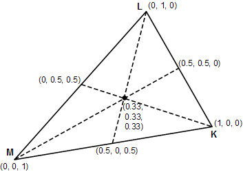
If the field is evaluated at a number of regular points and a grid is drawn between them, we can construct a set of hypothetical cubes with a single sample at each of its 8 vertices. By comparing the values at each vertex, it is trivial to determine the plane of intersection between the theoretical isosurface and the cubic sample volume. If properly evaluated, the local solutions for each sample volume will form integral parts of the global surface implicitly, without requiring any global information.

This is the basic theory behind the ubiquitous Marching Cubes algorithm, first published in 1987 and still commonly used today. While it is certainly battle-tested, there are a number of artifacts in the output geometry that can make surfaces appear rough. The generated triangles are also often non-uniform and narrow, leading to additional artifacts later in the rendering process. Perhaps a more pressing issue is the sheer number of cases to be evaluated. For every sample cell, there are 256 possible planar intersections. The fantastic implementation by Paul Bourke wisely recommends the use of a look-up table, pre-computing these cases. While this may work well in traditional implementations, it crumbles under the parallel architecture of modern GPUs. Graphics hardware tends to excel at executing large batches of identical instructions, but begins to falter as soon as complex conditional branching is involved and operations have to be evaluated individually. In my tests, I found that the look-up tables performed no better, if not worse than explicit evaluation, as the complier could not easily expand and unroll the program flow, and evaluation could not be easily batched. Bearing this in mind, we ideally need to implement a method with as few logical branches as possible.

Marching Tetrahedra is a variant of the Marching Cubes algorithm which divides each cube into 5 (or 6 for a slightly different topology) tetrahedra. By limiting our integral sample volume to four vertices instead of 8, the number of possible cases drops to 16. In my tests, I got a 16x performance improvement using this technique (though realized savings are heavily dependent on the hardware used), confirming our suspicions. Unfortunately, marching tetrahedra can have some strange surface features, and has a number of artifacts of its own, especially with dynamic sampling grids.

Because of this, I ended up settling on naive surface nets, a simple dual method which generates geometry spanning multiple voxel sample volumes. An excellent discussion of the differences between these three meshing algorithms can be found here. Perhaps my favorite advantage of this method is the relative uniformity of the output geometry. Surface nets tend to be smooth surfaces comprised of quads of relatively equal size. In addition, I find it easier to comprehend and follow than other meshing algorithms, as its use of look-up-tables, and possible cases is fairly limited.

Implementation Details

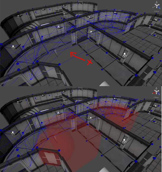
The sample grid is actually defined as a mesh, with a single disjoint vertex placed at each integral sample coordinate. These vertices aren’t actually drawn, but instead are used as input data to a series of shaders. Therefore, the shader can be considered to be executed “per-voxel”, with its only input being the coordinate of the minimum bounding corner. One disadvantage commonly seen in similar systems is a fundamental restriction on surface resolution due to a uniform sample grid. In order to skirt around this limitation, meshing is actually performed. In projected space, rather than world space, so each voxel is a truncated frustum similar to that of the camera, rather than a cube. This not only eliminates a few extra transformations in the shader code, but provides LoD implicitly by ensuring each output triangle is of a fixed pixel size, regardless of its distance to the camera.

Once the sample mesh was created, I used a simple density function for the potential field used by this system. It provides a good amount of flexibility, while still being simple to comprehend and implement. Each new source of “charge” added to the field would contribute additively to the overall potential. However, this quickly raises a concern! Each contributing charge must be evaluated at all sample locations, meaning our shader must, in some way, iterate through all visible charges! As stated earlier, branching and loops which cannot be unrolled can cause serious performance hiccups on most GPUs!

While I was at it, I also implemented a Vertex Pre-pass. Due to the nature of GPU parallelism, each voxel is evaluated in complete isolation. This has the unfortunate side-effect of solving for each voxel vertex position up to 6 times (once for each neighboring voxel). The surface net algorithm utilizes an interpolated surface vertex position, determined from the intersections of the surface and the sample volume. This interpolation can get expensive if repeated 6 times more than necessary! To remedy this, I instead do a pre-pass calculating the interpolated vertex position, and storing it as a normalized coordinate within the voxel in the pixel color of another texture. When the geometry stage builds triangles, it can simply look up the normalized vertex positions from this table, and spit them out as an offset from the voxel min coordinate!

The geometry shader stage is then fairly straightforward, reading in vertex positions, checking the case of the input voxel, looking up the vertex positions of its neighbors, and bridging the gap with a triangle.

Was it worth it?

Short answer, no.

I am extremely proud of the work I’ve done, and the end result is quite cool, but it’s not a solution I would recommend in a production setting. The additional complexity far outweighs any potential performance benefit, and maintainability, while not terrible, takes a hit as well. In addition, the geometry shader approach doesn’t work nearly as well as I had hoped. Geometry shaders are notoriously cache-unfriendly, and my implementation is no exception. Combine this with the rather unintuitive nature of working with on-GPU procedural geometry in a full-scale project, and you’ve got yourself a recipe for very unhappy engineers.

I think the concept of on-GPU surface meshing is fascinating, and I’m eager to look into Compute Shader implementations, but as it stands, the geometry stage is not the way to go.

I’ve made the source available on my GitHub if you’d like to check it out!

Keeping track of AssetBundles

Posted by andrewgotow on July 23, 2018

Sometimes it’s necessary to load and unload content at runtime. Games which take place in an expansive, explorable world, for instance, probably shouldn’t load the entire play-space up front. Every area, from the dankest catacomb to the loftiest castle, would need to be read from long-term storage and buffered into memory before the game could be played. Doing so would contribute to long load-times, and cause often insurmountable memory problems! Unfortunately, we don’t yet live in an era where a game-maker can reasonably expect players to have computers, consoles, and mobile devices capable of loading 30 gigabytes of dirt textures into memory.

The Unity game engine has long struggled with this problem. Multiple solutions for asset streaming exist, but all are far from perfect.

Perhaps the most convenient streaming solution in Unity is the Resources API. Added in the early days of the engine, it allows assets to be loaded and unloaded using two simple functions.

public static T Resources.Load<T>(string path);

public static void Resources.UnloadAsset(Object assetToUnload);

Look at that! It’s a simple interface which can easily be rolled into any custom asset management code you might want! It’s easy to read, intuitive, requires no special handling… and it’s terrible…

What’s wrong with Resources?

Unity itself strongly recommends against using the Resources API. To reiterate the official arguments, the Resources API makes it much more difficult to manage memory carefully. This might seem like a moot point, but on memory constrained platforms like Mobile devices, this can cause issues. Fragmentation of the heap is a very real concern, especially when loading and unloading many large objects. Additional, the official injunction omits the fact that the Resources API compiles all referenced resources into a single bundle at build-time, meaning the maximum total size of your resources are restricted to the maximum size of a single file on the user’s machine! On most machines, this will be either 2 or 4 gigabytes! Not nearly enough to represent that massive world you and your team have been planning!

So what’s the alternative?

Unity added an alternative method for streaming assets sometime in the late 2000’s known as “Asset Bundles“. AssetBundles are compressed archives of content which can be loaded and unloaded on the fly in your application. Games can even download AssetBundles from a server to perform partial updates, and pull down large chunks of data at a time (useful for games like MMOs, which can’t feasibly store the entire world at once).

Yes, AssetBundles are wonderful, but all that flexibility isn’t without its downsides. Long gone are the days of “Resources.Load()”. AssetBundles require a slew of management. Loading bundles, loading dependencies, shifting around manifests, and compulsively version-checking your data are unfortunate requirements of the system. To poorly paraphrase Uncle Ben from the 2002 film adaptation of Spider-Man, “With great interface flexibility, comes a need for specificity.”

What can be done?

The job of a programmer is one of abstraction. I set out to write a facade over the AssetBundle system as an “exploratory exercise.” Surely, there’s a way to keep track of assets, their dependencies, and their lifespans without having to manually modify each piece of code we write!

I decided to adapt a concept from the Objective-C runtime. Apple’s OSX and iOS SDKs contain a memory-managment system known as ARC (Automatic Reference Counting). Essentially, what ARC does is keep a counter running for every instance of an object in your application. When an object is referenced somewhere, that counter is incremented. When that reference goes out of scope, the counter is decremented. When the counter reaches zero, the object is destroyed.

This has the net effect of “automatically” keeping track of when an object is referenced, and when it is no longer needed, similar to the “garbage collection” systems present in many environments (including Unity’s .NET execution environment). Unlike Garbage Collection however, it tends to incur a less noticeable runtime performance cost, as instances are freed from memory continuously rather than in an occasional “clean up” pass. This is not without its downsides, but that’s another story for another post.

The important thing is that the theory can be applied to AssetBundles. Game assets are a good use case for a system like this. Assets must be loaded on demand, but in environments with limited memory, must be freed as soon as possible. Dependencies are also a very real concern. AssetBundles may depend on others for content, and it’s important to know which bundles can and can’t be unloaded safely during the execution of an application. I figured it was worth a shot, and spent a few hours looking into things…

Automatic Reference-Counted StreamedAsset API

The StreamedAsset API is fairly simple and not without its own set of issues, however as a first experiment, it does a solid job of mimicking the simplicity of the old “Resources” API.

First, I define a generic class called “StreamedAsset”. This class will act as a wrapper to handle reference-counting of an internally managed Object instance!

public sealed partial class StreamedAsset<AssetType> where AssetType : Object {

public readonly string bundleName;
public readonly string assetName;

public StreamedAsset(string bundleName, string assetName) {
this.bundleName = bundleName;
this.assetName = assetName;

ReferenceBundle(bundleName);
ReferenceAsset(assetName);
}

~StreamedAsset() {
DereferenceBundle(bundleName);
DereferenceAsset(assetName);
}

public static implicit operator AssetType(StreamedAsset<AssetType> streamedAsset) {
LoadAsset(streamedAsset.bundleName, streamedAsset.assetName);
return m_loadedAssets[streamedAsset.assetName] as AssetType;
}

}

First, a StreamedAsset contains a “bundleName” and “assetName” field. These fields contain the name of the AssetBundle containing the desired asset, and the name of that asset itself, respectively.

You’ll notice two lines in both the initializer, and finalizer of this class…

(De)ReferenceBundle(bundleName);
(De)ReferenceAsset(assetName);

These methods increment and decrement the reference counter for the bundle and asset within that bundle. This makes it externally impossible to construct an instance of “StreamedAsset” without updating the reference counters corresponding to the asset data. The finalizer is called automatically whenever this object is destroyed by the garbage collector, so our reference counters will be correctly decremented sometime after this object goes out of scope, whenever the runtime decides it’s safe to free unnecessary memory.

You’ll also notice the “Implicit Operator” towards the end of the definition. This is how we unwrap our StreamedAsset references. The implementation of this conversion operator means that they are implicitly convertible to the contained generic type. This allows StreamedAsset instances to be used identically to a traditional reference to our asset data.

// Works

renderer.material = new Material();

// Also works!

renderer.material = new StreamedAsset<Material>(“myBundle”, “matName”);

Included in this implicit operator is a call to the “LoadAsset” function. This function will do nothing if the object is loaded, but has the effect of lazily loading the asset in question. Therefore, StreamedAsset references can be instantiated, duplicated, and passed around the application without ever actually loading the asset from the AssetBundle! You can define a thousand references to a thousand assets, but until they’re actually used for something, they remain unloaded. Placing the lazy load function in the implicit unwrap operator also allows assets to be unloaded when they’re referenced, but not used (though this behavior is not implemented in this demo project).

Now, our asset exists, but what about the actual loading and unloading?

StreamedAsset Internals

I made the StreamedAsset API a partial class, allowing it to be separated into multiple files. While the management of asset data and the asset reference type should be contained in different places, the management should still be completely internal to the StreamedAsset type. They are fundamentally inseparable, and it should not be externally accessible!

public sealed partial class StreamedAsset<AssetType> {

private static SynchronizationContext m_unitySyncContext;

private static Dictionary<string, AssetBundle> m_loadedBundles = new Dictionary<string, AssetBundle>();
private static Dictionary<string, Object> m_loadedAssets = new Dictionary<string, Object>();

private static Dictionary<string, uint> m_bundleRefCount = new Dictionary<string, uint>();
private static Dictionary<string, uint> m_assetRefCount = new Dictionary<string, uint>();

static StreamedAsset() {
m_unitySyncContext = SynchronizationContext.Current;
}

private static void ReferenceAsset(string name) {
if (!m_assetRefCount.ContainsKey(name))
m_assetRefCount.Add(name, 0);
m_assetRefCount[name] ++;

}

private static void DereferenceAsset(string name) {
m_assetRefCount[name] –;

if (m_assetRefCount[name] <= 0) {
// Dereferencing is handled through finalizers, which are run on
// background threads. Execute the unloading on the Unity sync context.
m_unitySyncContext.Post(_ => {
UnloadAsset(name);
}, null);
}
}

private static void ReferenceBundle(string name) {
if (!m_bundleRefCount.ContainsKey(name))
m_bundleRefCount.Add(name, 0);
m_bundleRefCount[name] ++;

}

private static void DereferenceBundle(string name) {
m_bundleRefCount[name] –;

if (m_bundleRefCount[name] <= 0) {
// Dereferencing is handled through finalizers, which are run on
// background threads. Execute the unloading on the Unity sync context.
m_unitySyncContext.Post((context) => {
UnloadBundle(context as string);
}, name);
}
}

private static void LoadBundle(string bundleName) {
if (m_loadedBundles.ContainsKey(bundleName))
return;

var path = System.IO.Path.Combine(Application.streamingAssetsPath, bundleName);
var bundle = AssetBundle.LoadFromFile(path);
m_loadedBundles.Add(bundleName, bundle);
}

private static void UnloadBundle(string bundleName) {
var bundle = m_loadedBundles[bundleName];
m_loadedBundles.Remove(bundleName);

if (bundle != null) {
bundle.Unload(true);
}
}

private static void LoadAsset(string bundleName, string assetName) {
if (m_loadedAssets.ContainsKey(assetName))
return;

LoadBundle(bundleName);
var asset = m_loadedBundles[bundleName].LoadAsset(assetName);
m_loadedAssets.Add(assetName, asset);
}

private static void UnloadAsset(string assetName) {
var asset = m_loadedAssets[assetName];
m_loadedAssets.Remove(assetName);

// if (asset != null) {
// Resources.UnloadAsset(asset);
// }
Resources.UnloadUnusedAssets();
}
}

This portion of the StreamedAsset class does exactly what it looks like, implementing functions to load, and unload asset bundles, as well as method to increment and decrement reference counts.

An important thing to note is the use of a “SynchronizationContext” to unload assets. The finalizer for object instances in Unity is executed on a background thread dedicated to garbage collection. As a result, all functions called from a finalizer will be executed on this background thread. Unfortunately, Unity’s Scripting API is not thread-safe! The static initializer is therefore used to capture a reference to the SynchronizationContext of Unity’s main thread, and all requests to unload assets are handled through this context.

Another note is the use of the “Resources.UnloadUnusedAssets()” method. While the Resources API is deprecated, a number of asset management functions are still grouped under the “Resource” umbrella. “Resources.UnloadAsset()”, and “Resources.UnloadUnusedAssets()” can actually be used to unload assets loaded from AssetBundles. This is never explicitly documented, however it is supported, and is clearly intended functionality. In the example, “UnloadUnusedAssets()” is used because it also unloads the dependencies of the dereferenced asset. This function has large performance implications, and should probably not be called so liberally, but as stated earlier, is useful for prototyping.

That’s really all there is to it! A custom build script can be included to construct bundles of streamed assets for the target platform, and copy them into the StreamingAssets “magic directory”. From there, the StreamedAsset API can be used to load them on the fly without ever having to worry about the nitty gritty of managing references!

Room for Improvement!

This is clearly not a perfect solution! The first and foremost issue is that the lifecycle of a streamed asset is tied to the lifecycle of its “StreamedAsset” references, rather than the asset itself.

For example, assigning a implicitly converted StreamedAsset directly to a built-in Unity component will cause that asset to be unloaded as soon as garbage is collected. Assets must instead be maintained at a higher level than function-scope.

private StreamedAsset m_goodMat = new StreamedAsset<Material>(“myBundle”, “myMat”);

void Start() {

var badMat = new StreamedAsset<Material>(“myBundle”, “myMat”);

obj1.GetComponent<Renderer>().material = badMat

// At this point, “badMat” will go out of scope, and the material will become null at some point in the future.

obj2.GetComponent<Renderer>().material = m_goodMat;

// “m_goodMat” however will share the life cycle of this behaviour instance, and will persist for the lifespan of the object.

}

This is an unfortunate downside of the implicit conversion. As far as I can tell, it isn’t possible to retroactively embed automatic reference counting in the UnityEngine.Material instance itself, though a higher-level “management” solution warrants further investigation.

Final Words

I’m fairly happy with this little experiment, though I would advise against using it in a production environment without further testing. Regardless, I think reference-counted assets have potential in larger games. Not having to worry explicitly about asset loading and unloading trades performance for ease of use, but for many games, I’m willing to bet that’s a worthwhile trade. I’m curious to see what else can be done with a more “automatic” system such as this!

Air, Air Everywhere.

Posted by andrewgotow on September 20, 2016

Atmosphere Propagation Graph from Project: Commander

I have a personal game project I’ve been contributing to now and again, and it seems to be slowly devolving into a case study of over-engineering. Today I’d like to talk about an extremely robust, and extremely awesome system I got working in the past few days.

The game takes place aboard a spaceship engaged in combat with another ship. The player is responsible for issuing orders to the crew, selecting targets, distributing power to subsystems, and performing combat maneuvers, all from a first-person perspective aboard a windowless ship (after all, windows are structural weaknesses, and pretty much useless for targets more than 10 km away anyway).

Being a game that takes place in space, oxygen saturation and atmospheric pressure is obviously a constant concern, and presents several dangers to the player. I needed a way I could model this throughout the ship in a convincing, and efficient way.

What and Why?

We need a solution that handles a degree of granularity (ideally controllable by a designer), is very fast to update, and can handle the ambiguity of characters who may be transitioning between two areas. How can this be done?

Enter “Environment Probes”. A fairly common technique in computer graphics is the use of environment probes to capture and sample shading information in an area surrounding an object. Usually, these are used for reflections and lighting, allowing objects to blend between multiple static pre-baked reflections quickly rather than re-rendering a reflection at runtime. This same concept could be made to work with arbitrary volumetric data, rather than just lighting, and would cover many of the requirements of the atmosphere system!

So, let’s say that a designer can place “atmosphere probes” in the game world. Huzzah, all is well, but how can that data actually be used practically? Not only do we need to propagate values between probes, but characters need to be able to sample their environment for the current atmosphere values at their position, where there may or may not be a probe! Choosing just the nearest probe will introduce noticeable “seams” between areas, and still doesn’t easily give us the adjacency data we need to propagate values from one probe to the next!

“Light Probes” in the Unity game engine. An artist can place probes around the environment (shown as yellow spheres), and have the engine pre-calculate lighting information at each sample.

Let’s look at the Unity game engine for inspiration. One of their newer rendering features is “Light Probe Groups”, which is used for lighting objects as described above. Their mechanism is actually quite clever. They build a Delaunay tetrahedralization of hand-placed probes, resulting in a mesh defining a series of tetrahedral volumes. These volumes can then be used to sample the probes at each of the four vertices, and interpolate the lighting data for the volume between them! In theory, this doesn’t have to just be for light. By simply generalizing the concept, we could theoretically place probes for any volumetric data!

Let’s Get Graphic!

I spent the majority of the time building a triangulation framework based on Bowyer-Watson point insertion. Essentially, we iteratively add in vertices one at a time, and check whether the mesh is still a valid Delaunay triangulation with each insertion. If any triangle fails to meet those constraints after the new vertex is inserted, it’s removed from the mesh, and rebuilt. This algorithm is quite simple conceptually, and works relatively quickly, making it a great choice for this system. Once this was working, it was quite simple to flesh it out in the third dimension.

A simple Delaunay tetrahedralization of a series of “Atmosphere Probes”.

So now what? So far we have a volumetric mesh defined across a series of probe objects. What can we do with this?

Each probe has an attached “Atmosphere Probe” component which allows it to store properties about the air at that location. Pressure, oxygen saturation, temperature, you name it. This is nice in itself, but the mesh also gives us a huge amount of local information. For starters, it gives us a clear idea of which atmosphere probes are connected, and the distance between them. A few times every second, the atmosphere system will look at every edge in the graph and calculate the pressure difference between the two vertices it connects. Using the pressure difference, it will propagate atmosphere properties along that edge. We essentially treat each probe as a cell connected to its neighbors by edges, and design a fluid-dynamics simulation at a variable resolution. This means that the air at eye-level can be simulated accurately and used for all sorts of cool visual effects, while the simulation around the player’s ankles can be kept extremely coarse to avoid wasting precious iterations. By iterating through edges, we partially avoid the combinatorial explosion that would result from comparing every unique pair of graph vertices, and we can ensure that no cells will be “skipped over” when calculating flow.

Interpolation – Pretending To Know What We Don’t.

Now, how do we actually sample this data?! The probes are nice, but what if the player is standing near them, rather than on them? We want to smoothly interpolate data between these probes, so that we can sample the mesh volume at arbitrary locations. Here, we can dust off our old 2D friend, barycentric coordinates. Normally, we humans like to think in cartesian coordinates. We define a set of orthogonal directions as “Up”, “Forward”, and “Right”, and then express everything relative to those directions. “In front, and a little to the right of me…” but coordinate systems don’t always need to be this way! In theory, we could describe a location using any basis.

An example of a barycentric coordinate system. Each triplet shows the coordinates of that point within the triangle.

Barycentric coordinate systems define points relative to the positions of the vertices of any arbitrary simplex. So for a triangle, one could say “80% of vertex 1, 26% of vertex 2, and 53% of vertex 3”. Conveniently, these coordinates are also normalized, meaning that a point exactly at vertex 1 will be expressed as (1,0,0). We can therefore use these coordinates for interpolation between these vertices by performing a weighted sum of the values of all the vertices of the simplex, using their corresponding component of the coordinate vector of the sample point!

So, the value of the point at the center of the diagram would be equal to

x = 0.33M + 0.33L + 0.33K

or, the average of the values of each vertex!

By calculating the barycentric coordinates of the sample point within each tetrahedron, we can determine how to average the values of each corner to find the value of that point! For our application, by knowing which tetrahedron the player is in, we can simply find the coordinates of the player in barycentric space, and do a fancy average to determine the exact atmospheric properties at his or her position! By clamping and re-normalizing coordinates, this system will also handle extrapolation, meaning that, even if the player exits the volume of the graph, the sampled properties will still be fairly accurate!

Wait… you just said “by knowing which tetrahedron the player is in…” How do we do that? Well, we can use our mesh from before to calculate even more useful information! We can determine adjacency between tetrahedra by checking if they share any faces. If two tetrahedra share three vertices, we know they are adjacent along the face formed by those three vertices… wait, it gets better… remember we had barycentric coordinates for our sample point anyway. Barycentric coordinates are normalized, and “facing inward”, so if any of our coordinates are negative, we know that the sample point must be contained within the adjacent tetrahedron opposite the vertex for which the coordinate is negative.

We essentially get to know if our sample point is in another tetrahedron for “free”, and by doing some preprocessing, we can tell exactly WHICH tetrahedron that point is within for “free”.

https://gfycat.com/EachMessyFlatfish
In the final solution, the player maintains a “current tetrahedron” reference. Whenever the player’s coordinates within that tetrahedron go negative, we update that reference to be the tetrahedron opposite the vertex with the negative coordinates. As long as the player moves smoothly and doesn’t teleport (which isn’t possible in the game I was writing this for), this reference will always be correct, and the sampler will always be aware of the tetrahedron containing the player. If the player does teleport, it will only take a few frames for the current tetrahedron reference to “walk” its way through the graph and correct itself! I also implemented some graph bounding volume checks, so I can even create multiple separate atmosphere graphs, and have the player seamlessly walk between them!

Concavity!

The last step was ensuring that I could actually design levels the way I wanted. I quickly found that I was unable to properly design concave rooms! The tetrahedralization would build edges through walls, allowing airflow between separate rooms that should be blocked off from one-another. I didn’t want to do any geometric collision detection because that would quickly become more of a hassle, and fine-tuning doorways and staircases to allow air to flow through them is not something I wanted to bother with. Instead, I implemented “Subtraction Volumes”. Essentially a way for a level designer to hint to the graph system that a given space is impassible. Once the atmosphere graph is constructed, a post-pass runs through the tetrahedron data and removes all tetrahedra which intersect a subtraction volume. By placing them around the level, the designer can essentially cut out chunks of the graph where they see fit.

Notice in the first image there are edges spanning vertices on either side of what should be a wall. After sphere and box subtraction volumes are added, these edges are removed.

Looking Forward!

And that’s about it! Throwing that together, along with a simple custom editor in the Unity engine, I now have a great tool for representing volumetric data! In the future, I can generalize the system to represent other things, such as temperature or light-levels, and by saving the data used to calculate sample propagation, I can also determine the velocity of the air at any point for drawing cool particle effects or wind sound effects! For now, the system is finished, but who knows, maybe I’ll add more to it in the future 🙂

https://gfycat.com/ShamefulDearestBittern

Heatwave

Posted by andrewgotow on November 10, 2015

A few years back I worked on a Unity engine game for a school project, called “Distortion”. In this game, the player has a pair of scifi-magic gloves that allows him or her to bend space. I ended up writing some really neat visual effects for the game, but it never really went anywhere. This afternoon I found a question from a fellow Unity developer, asking how to make “heat ripple” effects for a jet engine, and I decided to clean up the visual effects and package them into a neat project so that others could use it too!

And so, Heatwave was born.

heatwave_flame_demo_gif

Heatwave is a post-processing effect for the Unity game engine that takes advantage of multi-camera rendering to make cool distortion effects easy! It does this by rendering a full-screen normal map in the scene using a specialized shader. This shader will render particle effects, UI elements, or overlay graphics together into a single map that is then used to calculate refractions!

The main render target is blitted to a fullscreen quad, and distorted by offsetting the UV coordinates during the copy based on the refraction vector calculated using the normal map, resulting in a nice realtime psuedo-refraction!

There are a few issues with this method, mainly that it doesn’t calculate “true” refractions. The effect is meant to look nice more than to make accurate calculations, so cool effects like refracting light around corners and computing caustics aren’t possible. The advantage however is that the effect operates in screen-space. The time required to render distortion is constant, and the cost of adding additional distortion sources is near zero, making it perfect for games, and situations where a large number of sources will be messing with light!

I’ve made a small asset-package so other Unity developers can download the sources and use them!

You can find the project on Github here!

Pulse Racer

Posted by andrewgotow on October 25, 2013

I’ve released my iOS App, Pulse Racer on the app store!

Pulse Racer is a rhythm based score-attack game, which requires the player to travel along a generated course and collect “notes” which are synchronized to music. Players are rated based on their ability to string together notes, and their final percentage at the end of each course.

I’m really quite happy with how the project turned out and, for me, having a polished app on the store is a huge accomplishment.

Technically this app was a big endeavor as well. I’ve had the idea floating around for a year or so, but was never able to properly execute it until now. Building courses based on music is more difficult than it seems at first glance. Perhaps the most challenging part was determining the positions of notes on the course. I used a spectral-flux based onset detection algorithm, which ran a Fourier transform over audio samples, converting them to the frequency domain. Next I calculated a net difference in each spectral band between samples using a rolling average. From this, I determined the change in acoustic energy for each sample window. From there, it was simply a matter of finding local maxima (locations where the energy peaked), and I had a reasonably reliable system. Other aspects of the course are generated from the intermediate steps. For instance, the large-scale contour of the course is based on the acoustic energy graph. The radius of the cylinder is based on the spectral flux over time, and so forth. Using these techniques together produced a fun, and challenging course for almost any song input into the game. This also allowed for tracks to be pre-processed, so that no complex calculations were done during the game, allowing for the absolute maximum frame rate.

https://vimeo.com/78839283

The music I used was made by an awesome artist I found online, F-777. He was kind enough to let me use a few of his songs as included sample tracks in the game, so that users did not need to generate their own to play. My experience working with him was a blast, and I’d highly recommend him to other developers looking for some good electro music.

Pulse Racer was a blast to work on, and was a wonderful learning experience for me. It is currently available on the App Store for $1.99 should you wish to play.

Pulse Racer Website

App Store Link

Andrew Gotow

An Online Portfolio

Category Archives: C#