Interior Mapping – Part 3

In part 2, we discussed a tangent-space implementation of the “interior mapping” technique, as well as the use of texture atlases for room interiors. In this post, we’ll briefly cover a quick and easy shadow approximation to add realism and depth to our rooms.

Hard Shadows

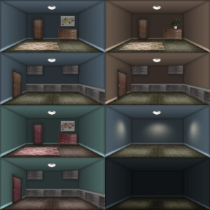
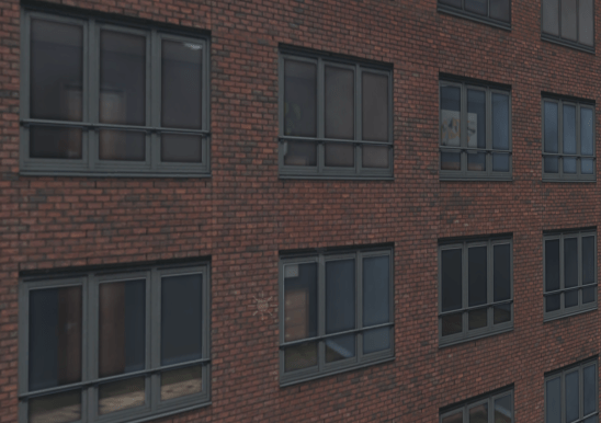
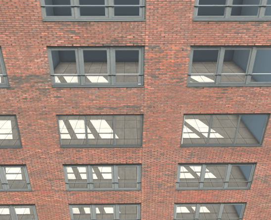
We have a cool shader which renders “rooms” inside of a building, but something is clearly missing. Our rooms aren’t effected by exterior light! While the current implementation looks great for night scenes where the lighting within the room can be baked into the unlit textures, it really leaves something to be desired when rendering a building in direct sunlight. In an ideal world, the windows into our rooms would cast soft shadows, which move across the floor as the angle of the sun changes.

Luckily, this effect is actually quite easy to achieve! Recall how we implemented the ray-box intersection in part 2. Each room is represented by a unit cube in tangent-space. The view ray is intersected with the cube, and the point of intersection is used to determine a coordinate in our room interior texture. As a byproduct of this calculation, the point of intersection in room-space is already known! We also currently represent windows using the alpha channel of the exterior texture. We can simply reuse this alpha channel as a “shadow mask”. Areas where the exterior is opaque are considered fully in shadow, since no light would enter the room through the solid wall. Areas where the exterior is transparent would be fully effected by light entering the room. If we can determine a sample coordinate, we can simply sample the exterior alpha channel to determine whether an interior fragment should be lit, or in shadow!

So, the task at hand: How do we determine the sample coordinate for our shadow mask? It’s actually trivially simple. If we cast the light ray backwards from the point of intersection between the view ray and the room volume, we can determine the point of intersection on the exterior wall, and use that position to sample our shadow texture!

Our existing effect is computed in tangent space. Because of this, all calculations are identical everywhere on the surface of the building. If we transform the incoming light direction into tangent space, any light shining into the room will always be more or less along the Z+ axis. Additionally, the room is axis-aligned, so the ray-plane intersection of the light ray and exterior wall can be simplified dramatically.

// This whole problem can be easily solved in 2D
// Determine the origin of the shadow ray. Since
// everything is axis-aligned, This is just the
// XY coordinate of the earlier ray-box intersection.
float2 sOri = roomPos.xy;

// Determine a 2D ray direction. This is the
// "XY per unit Z" of the light ray
float2 sDir = (-IN.tLightVec.xy / IN.tLightVec.z) * _RoomSize.z;

// Lastly, determine our shadow sample position. Since
// our sDir is unit-length along the Z axis, we can
// simply multiply by the depth of the fragment to
// determine the 2D offset of the final shadow coord!
float2 sPos = sOri + sDir * roomPos.z;


That’s about it! We can now scale the shadow coordinate to match the exterior wall texture, and boom! We have shadows.

Screen Shot 2019-02-27 at 11.42.23 AM.png

Soft Shadows

We have hard shadows up and running, and everything is looking great. What we’d really like is to have soft shadows. Typically, these are rendered with some sort of filtering, a blur, or a fancy technique like penumbral wedges. That’s not going to work here. We’re trying to reduce the expense of rendering interior details. We’re not using real geometry, so we can’t rely on any traditional techniques either. What we need to do is blur to our shadows, without actually performing a multi-sampled blur.

Like all good optimizations, we’ll start with an assumption. Our windows are a binary mask. They’re either fully transmissive, or fully opaque. In most cases this is how the effect will be used anyway, so the extra control isn’t a big loss. Now, with that out of the way, we can use the alpha channel of our exterior texture as something else!

Signed Distance Fields

Signed Distance Fields have been around for a very long time, and are often used to render crisp edges for low-resolution decals, as suggested in “Improved Alpha-Tested Magnification for Vector Textures and Special Effects”. Rather than storing the shadow mask itself in the alpha channel, we can store a new map where the alpha value represents the distance from the shadow mask’s borders.SDF Shadowmask.png

Now, a single sample returns not just whether a point is in shadow, but the distance to the edge of a shadow! If we want our shadows to have soft edges, we can switch from a binary threshold to a range of “shadow intensity”, still using only a single sample!

The smoothstep function is a perfect fit for our shadow sampling, remapping a range to 0-1, with some nice easing. We can also take the depth of the fragment within the room into account to emulate the softer shadows you see at a distance from a light source. Simply specify a shadow range based on the Z coordinate of the room point, and we’re finished!

Putting it all Together!

All together, our final shadow code looks like this.

#if defined(INTERIOR_USE_SHADOWS)
	// Cast a ray backwards, from the point in the room opposite
	// the direction of the light. Here, we're doing it in 2D,
	// since the room is in unit-space.
	float2 sOri = roomPos.xy;
	float2 sDir = (-IN.tLightVec.xy / IN.tLightVec.z) * _RoomSize.z;
	float2 sPos = sOri + sDir * roomPos.z;

	// Now, calculate shadow UVs. This is remapping from the
	// light ray's point of intersection on the near wall to the
	// exterior map.
	float2 shadowUV = saturate(sPos) * _RoomSize.xy;
	shadowUV *= _Workaround_MainTex_ST.xy + _Workaround_MainTex_ST.zw;
				
	// Finally, sample the shadow SDF, and simulate soft shadows
	// with a smooth threshold.
	fixed shadowDist = tex2D(_ShadowTex, shadowUV).a;
	fixed shadowThreshold = saturate(0.5 + _ShadowSoftness * (-roomPos.z * _RoomSize.z));
	float shadow = smoothstep(0.5, shadowThreshold, shadowDist);

	// Make sure we don't illuminate rooms facing opposite the light.
	shadow = lerp(shadow, 1, step(0, IN.tLightVec.z));

	// Finally, modify the output albedo with the shadow constant.
	iAlbedo.rgb = iAlbedo.rgb * lerp(1, _ShadowWeight, shadow);
#endif

https://gfycat.com/DangerousRectangularDungbeetle

And that’s all there is to it! Surprisingly simple, and wonderfully cheap to compute!

There’s still room for improvement. At the moment the shadow approximation supports only a single directional light source. This is fine for many applications, but may not work for games where the player is in control of a moving light source. Additionally, this directional light source is configured as a shader parameter, and isn’t pulled from the Unity rendering pipeline, so additional scripts will be necessary to ensure it stays in sync.

For deferred pipelines, it may be possible to use a multi-pass approach, and write the interior geometry directly into the G-buffers, allowing for fully accurate lighting, but shadows will still suffer the same concessions.

Still, I’m quite happy with the effect. Using relatively little math, it is definitely possible to achieve a great interior effect for cheap!

Interior Mapping – Part 2

In part 1, we discussed the requirements and rationale behind Interior Mapping. In this second part, we’ll discuss the technical implementation of what I’m calling (for lack of a better title) “Tangent-Space Interior Mapping”.

Coordinates and Spaces

In the original implementation, room volumes were defined in object-space or world-space. This is by far the easiest coordinate system to work in, but it quickly presents a problem! What about buildings with angled or curved walls? At the moment, the rooms are bounded by building geometry, which can lead to extremely small rooms in odd corners and uneven or truncated walls!

In reality, outer rooms are almost always aligned with the exterior of the building. Hallways rarely run diagonally and are seldom narrower at one end than the other! We would rather have all our rooms aligned with the mesh surface, and then extruded inward towards the “core” of the building.

Cylindrical Building

Curved rooms, just by changing the coordinate basis.

In order to do this, we can just look for an alternative coordinate system for our calculations which lines up with our surface (linear algebra is cool like that). Welcome to Tangent Space! Tangent space is already used elsewhere in shaders. Even wonder why normal-maps are that weird blue color? They actually represent a series of directions in tangent-space, relative to the orientation of the surface itself. Rather than “Forward”, a Z+ component normal map points “Outward”. We can simply perform the raycast in a different coordinate basis, and suddenly the entire problem becomes surface-relative in world-space, while still being axis-aligned in tangent space! A neat side-effect of this is that our room volumes now follow the curvature of the building, meaning that curved facades will render curved hallways running their length, and always have a full wall parallel to the building exterior.

While we’re at it, what if we used a non-normalized ray? Most of the time, a ray should have a normalized direction. “Forward” should have the same magnitude as “Right”. If we pre-scale our ray direction to match room dimensions, then we can simplify it out of the problem. So now, we’re performing a single raycast against a unit-sized axis-aligned cube!

Room Textures

The original publication called for separate textures for walls, floors, and ceilings. This works wonderfully, but I find it difficult to work with. Keeping these three textures in sync can get difficult, and atlasing multiple room textures together quickly becomes a pain. Alternative methods such as the one proposed by Zoe J Wood in “Interior Mapping Meets Escher” utilizes cubemaps, however this makes atlasing downright impossible, and introduces new constraints on the artists building interior assets.
interior_atlas
Andrew Willmott briefly touched on an alternative in “From AAA to Indie: Graphics R&D”, which used a pre-projected interior texture for the interior maps in SimCity. This was the format I decided to use for my implementation, as it is highly author-able, easy to work with, and provides results only slightly worse than full cubemaps. A massive atlas of room interiors can be constructed on a per-building basis, and then randomly selected. Buildings can therefore easily maintain a cohesive interior style with random variation using only a single texture resource.

Finally, The Code

I’ve excluded some of the standard Unity engine scaffolding, so as to not distract from the relevant code. You won’t be able to copy-paste this, but it should be easier to see what’s happening as a result.

v2f vert (appdata v) {
   v2f o;
   
   // First, let's determine a tangent basis matrix.
   // We will want to perform the interior raycast in tangent-space,
   // so it correctly follows building curvature, and we won't have to
   // worry about aligning rooms with edges.
   half tanSign = v.tangent.w * unity_WorldTransformParams.w;
   half3x3 objectToTangent = half3x3(
      v.tangent.xyz,
      cross(v.normal, v.tangent) * tanSign,
      v.normal);

   // Next, determine the tangent-space eye vector. This will be
   // cast into an implied room volume to calculate a hit position.
   float3 oEyeVec = v.vertex - WorldToObject(_WorldSpaceCameraPos);
   o.tEyeVec = mul(objectToTangent, oEyeVec);

   // The vertex position in tangent-space is just the unscaled
   // texture coordinate.
   o.tPos = v.uv;

   // Lastly, output the normal vertex data.
   o.vertex = UnityObjectToClipPos(v.vertex);
   o.uv = TRANSFORM_TEX(v.uv, _ExteriorTex);

   return o;
}

fixed4 frag (v2f i) : SV_Target {
   // First, construct a ray from the camera, onto our UV plane.
   // Notice the ray is being pre-scaled by the room dimensions.
   // By distorting the ray in this way, the volume can be treated
   // as a unit cube in the intersection code.
   float3 rOri = frac(float3(i.tPos,0) / _RoomSize);
   float3 rDir = normalize(i.tEyeVec) / _RoomSize;

   // Now, define the volume of our room. With the pre-scale, this
   // is just a unit-sized box.
   float3 bMin = floor(float3(i.tPos,-1));
   float3 bMax = bMin + 1;
   float3 bMid = bMin + 0.5;

   // Since the bounding box is axis-aligned, we can just find
   // the ray-plane intersections for each plane. we only 
   // actually need to solve for the 3 "back" planes, since the 
   // near walls of the virtual cube are "open".
   // just find the corner opposite the camera using the sign of
   // the ray's direction.
   float3 planes = lerp(bMin, bMax, step(0, rDir));
   float3 tPlane = (planes - rOri) / rDir;

   // Now, we know the distance to the intersection is simply
   // equal to the closest ray-plane intersection point.
   float tDist = min(min(tPlane.x, tPlane.y), tPlane.z);

   // Lastly, given the point of intersection, we can calculate
   // a sample vector just like a cubemap.
   float3 roomVec = (rOri + rDir * tDist) - bMid;
   float2 interiorUV = roomVec.xy * lerp(INTERIOR_BACK_PLANE_SCALE, 1, roomVec.z + 0.5) + 0.5;

#if defined(INTERIOR_USE_ATLAS)
   // If the room texture is an atlas of multiple variants, transform
   // the texture coordinates using a random index based on the room index.
   float2 roomIdx = floor(i.tPos / _RoomSize);
   float2 texPos = floor(rand(roomIdx) * _InteriorTexCount) / _InteriorTexCount;

   interiorUV /= _InteriorTexCount;
   interiorUV += texPos;
#endif

   // lastly, sample the interior texture, and blend it with an exterior!
   fixed4 interior = tex2D(_InteriorTex, interiorUV);
   fixed4 exterior = tex2D(_ExteriorTex, i.uv);

   return lerp(interior, exterior, exterior.a);
}

And that’s pretty much all there is to it! The code itself is actually quite simple and, while there are small visual artifacts, it provides a fairly convincing representation of interior rooms!


Interior + Exterior Blend
https://gfycat.com/FrankSoftAvocet


There’s definitely more room for improvement in the future. The original paper supported animated “cards” to represent people and furniture, and a more realistic illumination model may be desirable. Still, for an initial implementation, I think things came out quite well!

Interior Mapping – Part 1

Rendering convincing environments in realtime has always been difficult, especially for games which take place at a “human” scale. Games consist of a series of layered illusions and approximations, all working (hopefully) together to achieve a unified goal; to represent the world in which the game takes place. In the context of a simplified or fantastical world, this isn’t too bad. It’s a matter of creating a unified style and theme that feels grounded in the reality of the particular game. The fantastic narrative platformer “Thomas was Alone”, for example, arguably conveys a believable world using just shape and color. As soon as a game takes place in an approximation of our real world however, the cracks start to appear. There are a tremendous number of “details” in the real world. Subtle differences on seemingly identical surfaces that the eye can perceive, even if not consciously.

uncanny valley

This CG incarnation of Dwayne Johnson as the titular “Scorpion King” is a prime example of “The Uncanny Valley”

We as humans are exceptionally good at identifying visual phenomena, and more importantly, its absence. You may have heard this referred to as “The Uncanny Valley”; when something is too realistic to be considered cute or cartoony, but too unrealistic to look… right… It’s extremely important to include some representation of those “missing” pieces, even if they’re not 100% accurate in order to preserve the illusion.

While not nearly as noticeable at first glance, missing details in an environment are equally important to preserving the illusion of a living, breathing, virtual world.

Take, for example, this furniture store from GTA IV.

GTA Furniture Store.png

A nice looking furniture store, though something’s missing…

This is a very nice piece of environment art. It’s visually interesting, it fits the theme and location, and it seems cohesive within the world… though something is amiss. The view through the windows is clearly just a picture of a store, slapped directly onto the window pane, like a sticker on the glass! There’s no perspective difference between the individual windows on different parts of the facade. The view of the interior is always head-on, even if the camera is at an angle to the interior walls. This missing effect greatly weakens the illusion.

From this, the question arises…

How do we convey volume through a window, without creating tons of work for artists, or dramatically altering the production pipeline?

Shader Tricks!

The answer (as you may have guessed from the header) lies in shader trickery! To put it simply, Shaders are tiny programs which take geometric information as input, mush it around a bunch, and output a color. Our only concern is that the final output color looks correct in the scene. What happens in the middle frankly doesn’t matter much. If we offset the output colors, we can make it look like the input geometry is offset too! If outputs are offset non-uniformly, it can be made to appear as though the rendered image is skewed, twisted, or distorted in some way.

uncanny valley

If you’ve ever seen at 3D sidewalk art, you’ve seen a real-world implementation of parallax mapping.

The school of techniques collectively known as “Parallax Mapping” do just this. Input texture coordinates are offset based on the observer angle, and a per-texel “depth” value. By determining the point where our camera ray intersects the surface height-field, we can create what amounts to a 3D projection of an otherwise 2D image. “Learn OpenGL” provides an excellent technical explanation of parallax mapping if you’re curious.

While the theory is perfect for our needs, the methodology is lacking. Parallax mapping is not without its issues! Designed to be a general-purpose solution, it suffers from a number of visible artifacts when used in our specific case. It works best on smoother height-fields, for instance. Large differences in height between texels can create weird visual distortions! There are a number of alternatives to get around this issue (such as “Steep Parallax Mapping”), but many are iterative, and result in odd “step” artifacts as the ratio of depth to iteration count increases. In order to achieve a convincing volume for our buildings using an unmodified parallax shader, we’d need to use so many iterations that it would quickly become a performance nightmare.

Interior Mapping

Parallax mapping met nearly all of our criteria, but still wasn’t suitable for our application. Whenever a general solution fails, it’s usually a good idea to sit down and consider the simplest possible specific solution that will suffice.

Raymarch

For each point on the true geometry (blue), select a color at the point of intersection between the camera ray, and an imaginary room volume (red).

In our case, we want rectangular rooms inset into our surface. The keyword here is “rectangular”. The generality of parallax mapping means that an iterative numeric approach must be used, since there is no analytical way to determine where our camera ray intersects a general height-field. If we limit the problem to only boxes, then an exact solution is not only possible, but trivial! Furthermore, if these boxes are guaranteed to be axis-aligned, the computation becomes extremely simple! Then, it’s just a matter of mapping the point of intersection within our room volume to a texture, and outputting the correct color!

interior mapping example

Example of “Interior Mapping” from the original publication by Joost van Dongen.

Originally published in 2008, the now well known “Interior Mapping”, by Joost van Dongen seems like a prime candidate! In this approach, the facade of a building mesh is divided into “rooms”, and a raycast is performed for each texel. Then, the coordinate at the point of intersection between our camera ray and the room volume can be used to sample a set of “Room Textures”, and voila! This, similar to parallax mapping, offsets input texture coordinates to provide a projection of a wall, ceiling, and floor texture within each implicit “room volume”, resulting in a geometrically perfect representation of an interior without the added complexity of additional geometry and material work!

In part 2, we’ll discuss modifications to the original implementation for performance and quality-of-life improvements!

Abusing Blend Modes for Fun and Profit!

https://gfycat.com/ColdRemoteAndeancat
Today I decided to do a quick experiment.

Hardware “blend modes” have existed since the dawn of hardware-accelerated graphics. Primarily used for effects like transparency, they allow a developer to specify the way new colors are drawn into the buffer through a simple expression.

color = source * SrcFactor + destination * DstFactor

The final output color is the sum of a “source factor” term multiplied by the value output by the fragment shader, and a “destination factor” term multiplied by the color already in the buffer.

For example, if I wanted to simply add the new color into the scene, I could use blend modes of One One; Our coefficients would be negligible and we would end up with

color = source + destination

If I wanted a linear alpha blend between the source color and destination color, I could select the terms SrcAlpha, OneMinusSrcAlpha, which would perform a linear interpolation between the two colors.

But what happens when we have non-standard colors? Looking back at the blend expression, logic would dictate that we can express any two-term polynomial as long as the terms are independent, and the coefficients are one of the supported “blend factors”! By pre-loading our destination buffer with a value, the second term can be anything we need, and the alpha channel of our source can be packed with a coefficient to use as the destination factor if need be.

This realization got me thinking. “Subtract” blend modes aren’t explicitly supported in OpenGL, however a subtraction is simply the addition of a negative term. If our source term were negative, surely blend factors of One One would simply subtract the source from the destination color! That isn’t to say that this is guaranteed to work without issues! If the render target is a traditional 24 or 32-bit color buffer, then negative values may have undefined behavior! A subtraction by addition of a negative would only work assuming the sum is calculated independently somewhere in hardware, before it’s packed into the unsigned output buffer.

Under these assumptions, I set out to try my hand at a neat little trick. Rendering global object “thickness” in a single pass.

Why though?

Thickness is useful for a number of visual effects. Translucent objects, for example, could use the calculated thickness to approximate the degree to which light is absorbed along the path of the ray. Refraction could be more accurately approximated utilizing both incident, and emergent light calculations. Or, you could define the shape of a “fog volume” as an arbitrary mesh. It’s actually quite a useful thing to have!

Single pass global thickness maps

So here’s the theory. Every pixel in your output image is analogous to a ray cast into your scene. It can be thought of as a sweep backwards along the path of light heading towards the camera. What we really want to determine is the point where that ray enters and exits our object. Knowing these two points, we also essentially know the distance travelled through the volume along that ray.

It just so happens that we know both of these things! The projective-space position of a fragment must be calculated before a color can be written into a buffer, so we actually know the location of every fragment, or continuing the above analogy, ray intersection on the surface. This is also true of the emergent points, which all lie on the back-faces of our geometry! If we can find the distance the ray has traveled before entering our volume, and the distance the ray has traveled before exiting it, the thickness of the volume is just the difference of the two!

So how is this possible in a single pass? Well, normally when we render objects, we explicitly disable the “backfaces”; triangles pointing away from our camera. This typically speeds things up quite a bit, because backfaces almost certainly lie behind the visible portion of our model, and shading them is simply a waste of time. If we render them however, our fragment program will be executed both on the front and back faces! By writing the distance from the camera, or “depth” value as the color of our fragment, and negating it for front-faces, we can essentially output the “back minus front” thickness value we need!

DirectX provides a convenient semantic for fragment programs. float:VFACE. This value will be set to 1 when the fragment is part of a front-face, and -1 when the fragment is part of a back-face. Just render the depth, multiplied by the inverted value of the VFACE semantic, and we’ve got ourselves a subtraction!

Cull Off // disable front/back-face culling
Blend One One // perform additive (subtractive) blending
ZTest Off // disable z-testing, so backfaces aren’t occluded.

fixed4 frag (v2f i, fixed facing : VFACE) : SV_Target {
return -facing * i.depth;
}

Unity Implementation

From here, I just whipped up a quick “Camera Replacement Shader” to render all opaque objects in the scene using our thickness shader, and drew the scene to an off-screen “thickness buffer”. Then, in a post-effect, just sample the buffer, map it to a neat color ramp, and dump it to the screen! In just a few minutes, you can make a cool “thermal vision” effect!

Issues

The subtraction blend isn’t necessarily supported on all hardware. It relies on a lot of assumptions, and as such is probably not appropriate for real applications. Furthermore, this technique really only works on watertight meshes. Meshes with holes, or no back-faces will have a thickness of negative infinity, which is definitely going to cause some problems. There are also a number of “negative poisoning” artifacts, where the front-face doesn’t necessarily overlap a corresponding backface, causing brief pixel flickering. I think this occasional noise looks cool in the context of a thermal vision effect, but there’s a difference between a configurable “glitch” effect, and actual non-deterministic code!

Either way, I encourage everyone to play around with blend-modes! A lot of neat effects can be created with just the documented terms, but once you get into “probably unsafe” territory, things start to get really interesting!

GPU Isosurface Polygonalization

Isosurfaces are extremely useful when it comes to data visualization. From medical imaging to fluid flow analysis, they are an excellent tool for understanding complex volumetric data. Games have also adopted some of these techniques for their on purposes From the more rigid implementation in the ubiquitous game Minecraft to the Gels in Portal 2, these techniques serve the same basic purpose.

I wanted to try my hand at a general-purpose implementation, but before we dive into things, we must first answer a few basic questions.

What is an isosurface?

An isosurface can be thought of as the solution of a continuous function which produces a constant output in 3D. If you’re visualizing an electromagnetic field for example, you might generate an isosurface for a given potential, so you can easily determine its overall shape. This technique can be applied to other arbitrary values as well. Given CT scan data, a radiologist could construct an isosurface at the density of a specific type of tissue, extracting a 3D representation of bones or organs to view them separately, rather than having to manipulate a less intuitive stack of images.

What will we use this system for?

I don’t work in the medical field, nor would I trust the accuracy of my implementation when it comes to making a diagnosis. I work in entertainment and computer graphics, and as you would imagine, the requirements are quite different. Digital artists can already craft far better visuals than any procedure yet known; the real challenge is dynamic data. Physically simulated fluids, player-modifiable terrain, mechanics such as these present a significant challenge for traditional artists! What we really need is a generalized system for extracting and rendering isosurfaces in real time to fill in the gaps.

What are the requirements for such a system?

Given our previous use case, we can derive a few basic requirements. In no particular order…

  1. The system must be intuitive. Designers have other things to do besides tweaking simulation volumes and fiddling with configurations.
  2. The system must be flexible. If someone suggests a new mechanic which relies heavily on procedural geometry, it should be easy to get up and running.
  3. The system must be compatible. The latest experimental extensions are fun, but if you want to release something that anyone can enjoy, it needs to run on 5 year old hardware.
  4. The system must be fast. At 60 fps, you only have 16ms to render everything in your game. We can’t spend 10 of that drawing a special effect.

Getting Started!

Let’s look at requirement no. 4 first. Like many problems in computing, surface polygonalization can be broken down into repeated instances of much smaller problems. At the end of the day, the desired output is a series of interconnected polygons which appear to make up a complex surface. If each of these component polygons is accounted for separately, we can dramatically reduce the scope of the problem. Instead of generating a polygonal surface, we are now generating a single polygon, which is a much less daunting task. As with any discretization process, it is necessary to define a regular sample interval at which our continuous function will be evaluated. In the simplest 3D case, this will take the form of a regular grid of cells, and each of these cells will form a single polygon. Suddenly, this polygonalization process becomes massively parallel. With this new outlook, the problem becomes a perfect fit for standard graphics hardware!

For compatibility, I chose to implement this functionality in the Geometry Shader stage of the rendering pipeline, as it allows for the creation of arbitrary geometry given some basic input data. A Compute Shader would almost definitely be a better option in terms of performance and maintainability, but my primary development system is OSX, which presents a number of challenges when it comes to the use of Compute Shaders. I intend to update this project in the future, once Compute Shaders become more common.

If the field is evaluated at a number of regular points and a grid is drawn between them, we can construct a set of hypothetical cubes with a single sample at each of its 8 vertices. By comparing the values at each vertex, it is trivial to determine the plane of intersection between the theoretical isosurface and the cubic sample volume. If properly evaluated, the local solutions for each sample volume will form integral parts of the global surface implicitly, without requiring any global information.

This is the basic theory behind the ubiquitous Marching Cubes algorithm, first published in 1987 and still commonly used today. While it is certainly battle-tested, there are a number of artifacts in the output geometry that can make surfaces appear rough. The generated triangles are also often non-uniform and narrow, leading to additional artifacts later in the rendering process. Perhaps a more pressing issue is the sheer number of cases to be evaluated. For every sample cell, there are 256 possible planar intersections. The fantastic implementation by Paul Bourke wisely recommends the use of a look-up table, pre-computing these cases. While this may work well in traditional implementations, it crumbles under the parallel architecture of modern GPUs. Graphics hardware tends to excel at executing large batches of identical instructions, but begins to falter as soon as complex conditional branching is involved and operations have to be evaluated individually. In my tests, I found that the look-up tables performed no better, if not worse than explicit evaluation, as the complier could not easily expand and unroll the program flow, and evaluation could not be easily batched. Bearing this in mind, we ideally need to implement a method with as few logical branches as possible.

Marching Tetrahedra is a variant of the Marching Cubes algorithm which divides each cube into 5 (or 6 for a slightly different topology) tetrahedra. By limiting our integral sample volume to four vertices instead of 8, the number of possible cases drops to 16. In my tests, I got a 16x performance improvement using this technique (though realized savings are heavily dependent on the hardware used), confirming our suspicions. Unfortunately, marching tetrahedra can have some strange surface features, and has a number of artifacts of its own, especially with dynamic sampling grids.

Because of this, I ended up settling on naive surface nets, a simple dual method which generates geometry spanning multiple voxel sample volumes. An excellent discussion of the differences between these three meshing algorithms can be found here. Perhaps my favorite advantage of this method is the relative uniformity of the output geometry. Surface nets tend to be smooth surfaces comprised of quads of relatively equal size. In addition, I find it easier to comprehend and follow than other meshing algorithms, as its use of look-up-tables, and possible cases is fairly limited.

Implementation Details

Isosurface_Sample.png

The sample grid is actually defined as a mesh, with a single disjoint vertex placed at each integral sample coordinate. These vertices aren’t actually drawn, but instead are used as input data to a series of shaders. Therefore, the shader can be considered to be executed “per-voxel”, with its only input being the coordinate of the minimum bounding corner. One disadvantage commonly seen in similar systems is a fundamental restriction on surface resolution due to a uniform sample grid. In order to skirt around this limitation, meshing is actually performed. In projected space, rather than world space, so each voxel is a truncated frustum similar to that of the camera, rather than a cube. This not only eliminates a few extra transformations in the shader code, but provides LoD implicitly by ensuring each output triangle is of a fixed pixel size, regardless of its distance to the camera.

Once the sample mesh was created, I used a simple density function for the potential field used by this system. It provides a good amount of flexibility, while still being simple to comprehend and implement. Each new source of “charge” added to the field would contribute additively to the overall potential.  However, this quickly raises a concern! Each contributing charge must be evaluated at all sample locations, meaning our shader must, in some way, iterate through all visible charges! As stated earlier, branching and loops which cannot be unrolled can cause serious performance hiccups on most GPUs!

While I was at it, I also implemented a Vertex Pre-pass. Due to the nature of GPU parallelism, each voxel is evaluated in complete isolation. This has the unfortunate side-effect of solving for each voxel vertex position up to 6 times (once for each neighboring voxel). The surface net algorithm utilizes an interpolated surface vertex position, determined from the intersections of the surface and the sample volume. This interpolation can get expensive if repeated 6 times more than necessary! To remedy this, I instead do a pre-pass calculating the interpolated vertex position, and storing it as a normalized coordinate within the voxel in the pixel color of another texture. When the geometry stage builds triangles, it can simply look up the normalized vertex positions from this table, and spit them out as an offset from the voxel min coordinate!

The geometry shader stage is then fairly straightforward, reading in vertex positions, checking the case of the input voxel, looking up the vertex positions of its neighbors, and bridging the gap with a triangle.

Was it worth it?

Short answer, no.

I am extremely proud of the work I’ve done, and the end result is quite cool, but it’s not a solution I would recommend in a production setting. The additional complexity far outweighs any potential performance benefit, and maintainability, while not terrible, takes a hit as well. In addition, the geometry shader approach doesn’t work nearly as well as I had hoped. Geometry shaders are notoriously cache-unfriendly, and my implementation is no exception. Combine this with the rather unintuitive nature of working with on-GPU procedural geometry in a full-scale project, and you’ve got yourself a recipe for very unhappy engineers.

I think the concept of on-GPU surface meshing is fascinating, and I’m eager to look into Compute Shader implementations, but as it stands, the geometry stage is not the way to go.

I’ve made the source available on my GitHub if you’d like to check it out!

Keeping track of AssetBundles

Sometimes it’s necessary to load and unload content at runtime. Games which take place in an expansive, explorable world, for instance, probably shouldn’t load the entire play-space up front. Every area, from the dankest catacomb to the loftiest castle, would need to be read from long-term storage and buffered into memory before the game could be played. Doing so would contribute to long load-times, and cause often insurmountable memory problems! Unfortunately, we don’t yet live in an era where a game-maker can reasonably expect players to have computers, consoles, and mobile devices capable of loading 30 gigabytes of dirt textures into memory.

The Unity game engine has long struggled with this problem. Multiple solutions for asset streaming exist, but all are far from perfect.

Perhaps the most convenient streaming solution in Unity is the Resources API. Added in the early days of the engine, it allows assets to be loaded and unloaded using two simple functions.

public static T Resources.Load<T>(string path);

public static void Resources.UnloadAsset(Object assetToUnload);

Look at that! It’s a simple interface which can easily be rolled into any custom asset management code you might want! It’s easy to read, intuitive, requires no special handling… and it’s terrible…

What’s wrong with Resources?

Unity itself strongly recommends against using the Resources API. To reiterate the official arguments, the Resources API makes it much more difficult to manage memory carefully. This might seem like a moot point, but on memory constrained platforms like Mobile devices, this can cause issues. Fragmentation of the heap is a very real concern, especially when loading and unloading many large objects. Additional, the official injunction omits the fact that the Resources API compiles all referenced resources into a single bundle at build-time, meaning the maximum total size of your resources are restricted to the maximum size of a single file on the user’s machine! On most machines, this will be either 2 or 4 gigabytes! Not nearly enough to represent that massive world you and your team have been planning!

So what’s the alternative?

Unity added an alternative method for streaming assets sometime in the late 2000’s known as “Asset Bundles“. AssetBundles are compressed archives of content which can be loaded and unloaded on the fly in your application. Games can even download AssetBundles from a server to perform partial updates, and pull down large chunks of data at a time (useful for games like MMOs, which can’t feasibly store the entire world at once).

Yes, AssetBundles are wonderful, but all that flexibility isn’t without its downsides. Long gone are the days of “Resources.Load()”. AssetBundles require a slew of management. Loading bundles, loading dependencies, shifting around manifests, and compulsively version-checking your data are unfortunate requirements of the system. To poorly paraphrase Uncle Ben from the 2002 film adaptation of Spider-Man, “With great interface flexibility, comes a need for specificity.”

What can be done?

The job of a programmer is one of abstraction. I set out to write a facade over the AssetBundle system as an “exploratory exercise.” Surely, there’s a way to keep track of assets, their dependencies, and their lifespans without having to manually modify each piece of code we write!

I decided to adapt a concept from the Objective-C runtime. Apple’s OSX and iOS SDKs contain a memory-managment system known as ARC (Automatic Reference Counting). Essentially, what ARC does is keep a counter running for every instance of an object in your application. When an object is referenced somewhere, that counter is incremented. When that reference goes out of scope, the counter is decremented. When the counter reaches zero, the object is destroyed.

This has the net effect of “automatically” keeping track of when an object is referenced, and when it is no longer needed, similar to the “garbage collection” systems present in many environments (including Unity’s .NET execution environment). Unlike Garbage Collection however, it tends to incur a less noticeable runtime performance cost, as instances are freed from memory continuously rather than in an occasional “clean up” pass. This is not without its downsides, but that’s another story for another post.

The important thing is that the theory can be applied to AssetBundles. Game assets are a good use case for a system like this. Assets must be loaded on demand, but in environments with limited memory, must be freed as soon as possible. Dependencies are also a very real concern. AssetBundles may depend on others for content, and it’s important to know which bundles can and can’t be unloaded safely during the execution of an application. I figured it was worth a shot, and spent a few hours looking into things…

Automatic Reference-Counted StreamedAsset API

The StreamedAsset API is fairly simple and not without its own set of issues, however as a first experiment, it does a solid job of mimicking the simplicity of the old “Resources” API.

First, I define a generic class called “StreamedAsset”. This class will act as a wrapper to handle reference-counting of an internally managed Object instance!

public sealed partial class StreamedAsset<AssetType> where AssetType : Object {

public readonly string bundleName;
public readonly string assetName;

public StreamedAsset(string bundleName, string assetName) {
this.bundleName = bundleName;
this.assetName = assetName;

ReferenceBundle(bundleName);
ReferenceAsset(assetName);
}

~StreamedAsset() {
DereferenceBundle(bundleName);
DereferenceAsset(assetName);
}

public static implicit operator AssetType(StreamedAsset<AssetType> streamedAsset) {
LoadAsset(streamedAsset.bundleName, streamedAsset.assetName);
return m_loadedAssets[streamedAsset.assetName] as AssetType;
}

}

First, a StreamedAsset contains a “bundleName” and “assetName” field. These fields contain the name of the AssetBundle containing the desired asset, and the name of that asset itself, respectively.

You’ll notice two lines in both the initializer, and finalizer of this class…

 (De)ReferenceBundle(bundleName);
(De)ReferenceAsset(assetName);

These methods increment and decrement the reference counter for the bundle and asset within that bundle. This makes it externally impossible to construct an instance of “StreamedAsset” without updating the reference counters corresponding to the asset data. The finalizer is called automatically whenever this object is destroyed by the garbage collector, so our reference counters will be correctly decremented sometime after this object goes out of scope, whenever the runtime decides it’s safe to free unnecessary memory.

You’ll also notice the “Implicit Operator” towards the end of the definition. This is how we unwrap our StreamedAsset references. The implementation of this conversion operator means that they are implicitly convertible to the contained generic type. This allows StreamedAsset instances to be used identically to a traditional reference to our asset data.

// Works

renderer.material = new Material();

// Also works!

renderer.material = new StreamedAsset<Material>(“myBundle”, “matName”);

Included in this implicit operator is a call to the “LoadAsset” function. This function will do nothing if the object is loaded, but has the effect of lazily loading the asset in question. Therefore, StreamedAsset references can be instantiated, duplicated, and passed around the application without ever actually loading the asset from the AssetBundle! You can define a thousand references to a thousand assets, but until they’re actually used for something, they remain unloaded.  Placing the lazy load function in the implicit unwrap operator also allows assets to be unloaded when they’re referenced, but not used (though this behavior is not implemented in this demo project).

Now, our asset exists, but what about the actual loading and unloading?

StreamedAsset Internals

I made the StreamedAsset API a partial class, allowing it to be separated into multiple files. While the management of asset data and the asset reference type should be contained in different places, the management should still be completely internal to the StreamedAsset type. They are fundamentally inseparable, and it should not be externally accessible!

public sealed partial class StreamedAsset<AssetType> {

private static SynchronizationContext m_unitySyncContext;

private static Dictionary<string, AssetBundle> m_loadedBundles = new Dictionary<string, AssetBundle>();
private static Dictionary<string, Object> m_loadedAssets = new Dictionary<string, Object>();

private static Dictionary<string, uint> m_bundleRefCount = new Dictionary<string, uint>();
private static Dictionary<string, uint> m_assetRefCount = new Dictionary<string, uint>();

static StreamedAsset() {
m_unitySyncContext = SynchronizationContext.Current;
}

private static void ReferenceAsset(string name) {
if (!m_assetRefCount.ContainsKey(name))
m_assetRefCount.Add(name, 0);
m_assetRefCount[name] ++;

}

private static void DereferenceAsset(string name) {
m_assetRefCount[name] –;

if (m_assetRefCount[name] <= 0) {
// Dereferencing is handled through finalizers, which are run on
// background threads. Execute the unloading on the Unity sync context.
m_unitySyncContext.Post(_ => {
UnloadAsset(name);
}, null);
}
}

private static void ReferenceBundle(string name) {
if (!m_bundleRefCount.ContainsKey(name))
m_bundleRefCount.Add(name, 0);
m_bundleRefCount[name] ++;

}

private static void DereferenceBundle(string name) {
m_bundleRefCount[name] –;

if (m_bundleRefCount[name] <= 0) {
// Dereferencing is handled through finalizers, which are run on
// background threads. Execute the unloading on the Unity sync context.
m_unitySyncContext.Post((context) => {
UnloadBundle(context as string);
}, name);
}
}

private static void LoadBundle(string bundleName) {
if (m_loadedBundles.ContainsKey(bundleName))
return;

var path = System.IO.Path.Combine(Application.streamingAssetsPath, bundleName);
var bundle = AssetBundle.LoadFromFile(path);
m_loadedBundles.Add(bundleName, bundle);
}

private static void UnloadBundle(string bundleName) {
var bundle = m_loadedBundles[bundleName];
m_loadedBundles.Remove(bundleName);

if (bundle != null) {
bundle.Unload(true);
}
}

private static void LoadAsset(string bundleName, string assetName) {
if (m_loadedAssets.ContainsKey(assetName))
return;

LoadBundle(bundleName);
var asset = m_loadedBundles[bundleName].LoadAsset(assetName);
m_loadedAssets.Add(assetName, asset);
}

private static void UnloadAsset(string assetName) {
var asset = m_loadedAssets[assetName];
m_loadedAssets.Remove(assetName);

// if (asset != null) {
//  Resources.UnloadAsset(asset);
// }
Resources.UnloadUnusedAssets();
}
}

This portion of the StreamedAsset class does exactly what it looks like, implementing functions to load, and unload asset bundles, as well as method to increment and decrement reference counts.

An important thing to note is the use of a “SynchronizationContext” to unload assets. The finalizer for object instances in Unity is executed on a background thread dedicated to garbage collection. As a result, all functions called from a finalizer will be executed on this background thread. Unfortunately, Unity’s Scripting API is not thread-safe! The static initializer is therefore used to capture a reference to the SynchronizationContext of Unity’s main thread, and all requests to unload assets are handled through this context.

Another note is the use of the “Resources.UnloadUnusedAssets()” method. While the Resources API is deprecated, a number of asset management functions are still grouped under the “Resource” umbrella. “Resources.UnloadAsset()”, and “Resources.UnloadUnusedAssets()” can actually be used to unload assets loaded from AssetBundles. This is never explicitly documented, however it is supported, and is clearly intended functionality. In the example, “UnloadUnusedAssets()” is used because it also unloads the dependencies of the dereferenced asset. This function has large performance implications, and should probably not be called so liberally, but as stated earlier, is useful for prototyping.

That’s really all there is to it! A custom build script can be included to construct bundles of streamed assets for the target platform, and copy them into the StreamingAssets “magic directory”. From there, the StreamedAsset API can be used to load them on the fly without ever having to worry about the nitty gritty of managing references!

Room for Improvement!

This is clearly not a perfect solution! The first and foremost issue is that the lifecycle of a streamed asset is tied to the lifecycle of its “StreamedAsset” references, rather than the asset itself.

For example, assigning a implicitly converted StreamedAsset directly to a built-in Unity component will cause that asset to be unloaded as soon as garbage is collected. Assets must instead be maintained at a higher level than function-scope.

private StreamedAsset m_goodMat = new StreamedAsset<Material>(“myBundle”, “myMat”);

void Start() {

var badMat = new StreamedAsset<Material>(“myBundle”, “myMat”);

obj1.GetComponent<Renderer>().material = badMat

// At this point, “badMat” will go out of scope, and the material will become null at some point in the future.

obj2.GetComponent<Renderer>().material = m_goodMat;

// “m_goodMat” however will share the life cycle of this behaviour instance, and will persist for the lifespan of the object.

}

This is an unfortunate downside of the implicit conversion. As far as I can tell, it isn’t possible to retroactively embed automatic reference counting in the UnityEngine.Material instance itself, though a higher-level “management” solution warrants further investigation.

Final Words

I’m fairly happy with this little experiment, though I would advise against using it in a production environment without further testing. Regardless, I think reference-counted assets have potential in larger games. Not having to worry explicitly about asset loading and unloading trades performance for ease of use, but for many games, I’m willing to bet that’s a worthwhile trade. I’m curious to see what else can be done with a more “automatic” system such as this!

Messing With Shaders – Realtime Procedural Foliage


ivy_close.png
The programmable rendering pipeline is perhaps one of the largest advances in the history of realtime computer graphics. Before its introduction, graphics libraries like OpenGL and DirectX were limited to the “fixed function pipeline”, a programmer would shove in geometric data, and the application would draw it however it saw fit. Developers had little to no control over the output of their application beyond a few “render mode” settings. This was fine for rendering relatively simple scenes, solid objects, and simplistic lighting, but as visual fidelity increased and hardware become more powerful it quickly became necessary to allow for a more customizable rendering.

The process of rendering a 3D object in the modern programmable pipeline is typically broken down into a number of steps. Data is copied into fast-access graphics memory, then transformed through a series of stages before the graphics hardware eventually rasterizes that data to the display. In its most basic form, there are two of these stages the developer can customize. The “Vertex Program” manipulates data on a per-vertex level, such as positions and texture coordinates, before handing the results on to the “Fragment Program”, which is responsible for determining the properties of a given fragment (like a pixel containing more than just color information). The addition of just these two stages opened the floodgates for interesting visual effects. Approximating reflections for metallic objects, cel-shading effects for cartoon characters, and more! Since then, even more optional stages have been inserted into the pipeline for an even greater variety of effects.

I’ve spent a considerable amount of time experimenting with vertex and fragment programs in the past, but this week I decided to spend a few hours working with the other, less common stages, mainly “Geometry Programs”. Geometry programs are a more recent innovation, and have only began to see extensive use in the last decade or so. They essentially allow developers to not only modify vertex data as it’s received, but to construct entirely new vertices based on the input primitives (triangles, quads, etc.) As you can easily imagine, this presents incredible potential for new effects, and is something I personally would like to become more experienced with.

In four or five hours, I managed to write a relatively complex effect, and the rest of this post will detail, at a high level, what I did to achieve it.

ivy_distant.png

Procedurally generated geometry for ivy growing on a simple building.

This is my procedural Ivy shader. It is a relatively simple two-pass effect which will apply artist-configurable ivy to any surface. What sets this effect apart from those I’ve written in the past is that it actually constructs new geometry to add 3D leaves to the surface extremely efficiently.

One of the major technical issues when it comes to rendering things like foliage is that the level of geometric detail required to accurately represent leaves is quite high. While a digital environment artist could use a 3D modeling program to add in hundreds of individual leaves, this is not necessarily a good use of their time. Furthermore, it quickly becomes unmaintainable if anyone decides that the position, density, or style of foliage should change in the future. I don’t know about you, but I don’t want to be the one to have to tell a team of environment artists that all of the ivy in an entire game needs to be slightly different. In this situation, the key is to work smarter, not harder. While procedural art is often controversial in the game industry, I think most developers would agree that artist-directed procedural techniques are an invaluable tool.

Ivy_Shader_Steps.png
First and foremost, my foliage effect is composed of two separate rendering passes. First, a triplanar-mapped base texture is blended onto the object based on the desired density of the ivy. This helps to make the foliage feel much more dense, and helps to hide the seams where the leaves meet the base geometry.

Next in a second rendering pass, the geometry program transforms every input triangle into a set of quads lying on that triangle with a uniform, psuedo-random distribution. First, it is necessary to determine the number of leaf quads to generate. In order to maintain a consistent density of leaf geometry, the surface area of the triangle is calculated quickly using the “half cross-product formula”, and is then multiplied by the desired number of leaves per square meter of surface area. Then, for each of these leaves, a random sample point on the triangle is picked, and a triangle strip is emitted. It does this by sampling a noise function seeded with the world-space centroid of the triangle and the index of the leaf quad being generated. These noise values are then used to generate barycentric coordinates, which in turn are used to interpolate the position and normal of the triangle at that point, essentially returning a random world-space position and its corresponding normal vector.

Now, all that’s needed is to determine the orientation of the leaf, and output the correct triangle-strip primitive. Even this is relatively simple. By using the world-space surface normal and world “up” vector, a simple “change of vector basis” matrix is constructed. Combining this with a slightly randomized scale factor, and a small offset to orientation (to add greater variety to patches of leaves), we can transform normalized quad vertices into the exact world-space positions we want for our leaves!

...

// Defines a unit-size square quad with its base at the origin. doing
// this allows for very easy scaling and positioning in the next steps.
static const float3 quadVertices[4] = {
   float3(-0.5, 0.0, 0.0),
   float3( 0.5, 0.0, 0.0),
   float3(-0.5, 0.0, 1.0),
   float3( 0.5, 0.0, 1.0)
};

...

// IN THE GEOMETRY SHADER
// Change of basis matrix converts from XYZ space to leaf-space
float3x3 leafBasis = float3x3(
   leafX.x, leafY.x, leafZ.x,
   leafX.y, leafY.y, leafZ.y,
   leafX.z, leafY.z, leafZ.z
);

// constructs a random rotation matrix from Euler angles in the range 
// (-10,10) using wPos as a seed value.
float3x3 leafJitter = randomRotationMatrix(wPos, 10);

// Combine the basis matrix by the random rotation matrix to get the
// complete leaf transformation. Note, we could use a 4x4 matrix here
// and incorporate the translation as well, but it's easier to just add
// the world position as an offset in the final step.
float3x3 leafMatrix = mul(leafBasis, leafJitter);

// lastly, we can just output four vertices in a triangle strip
// to form a simple quad, and we'll be on our merry way.
for ( int i = 0; i < 4; i ++ ) {
   FS_INPUT v;
   v.vertex = UnityWorldToClipPos( 
      float4( mul(leafMatrix, quadVertices[i] * scale), 1) + wPos 
   );
   triStream.Append(v);
}

At this point, the meat of the work is done! We’ve got a geometry shader outputting quads on our surface. The last thing needed is to texture them, and it works!

Configuration!

I briefly touched on artist-configurable effects in the introduction, and I’d like to quickly address that too. I opted to go with the simplest solution I could think of, and it ended up being incredibly effective.

venus_vertex_weights.png

Configuring procedural geometry using painted vertex weights.

The density and location of ivy is controlled through painted vertex-colors. This allows artists to simply paint sections of their model they would like to be covered in foliage, and the shader will use this to weight the density and distribution of the procedural geometry. This way, an environment artist could use the tools they’re familiar with to quickly sketch out what parts of a model they would like to be effected by the shader. It will take an experienced artist less than a minute to get a rough draft working in-engine, and changes to the foliage can be made just as quickly!

At the moment, only the density of the foliage is mapped this way (All other parameters are uniform material properties), but I intend to expand the variety of properties which can be expressed this way, allowing for greater control over the final look of the model.

TODOs!

This ended up being an extremely informative project, but there are many things still left to do! For one, the procedural foliage does not take lighting into account. I built this effect in the Unity game engine, and opted out of using the standard “Surface Shader” code-generation system, which while very useful in 99% of cases, is extremely limiting in situations such as this. I would also like to improve the resolution of leaf geometry, applying adaptive runtime tessellation to the generated primitives in order to give them a slight curve, rather than displaying flat billboards. Other things, such as color variation on leaves could go a long way to improving the effect, but for now I’m quite satisfied with how it went!

Whelp, on to the next one!


Air, Air Everywhere.

atmosphere_graph

Atmosphere Propagation Graph from Project: Commander


I have a personal game project I’ve been contributing to now and again, and it seems to be slowly devolving into a case study of over-engineering. Today I’d like to talk about an extremely robust, and extremely awesome system I got working in the past few days.

The game takes place aboard a spaceship engaged in combat with another ship. The player is responsible for issuing orders to the crew, selecting targets, distributing power to subsystems, and performing combat maneuvers, all from a first-person perspective aboard a windowless ship (after all, windows are structural weaknesses, and pretty much useless for targets more than 10 km away anyway).

Being a game that takes place in space, oxygen saturation and atmospheric pressure is obviously a constant concern, and presents several dangers to the player. I needed a way I could model this throughout the ship in a convincing, and efficient way.


What and Why?

We need a solution that handles a degree of granularity (ideally controllable by a designer), is very fast to update, and can handle the ambiguity of characters who may be transitioning between two areas. How can this be done?

Enter “Environment Probes”. A fairly common technique in computer graphics is the use of environment probes to capture and sample shading information in an area surrounding an object. Usually, these are used for reflections and lighting, allowing objects to blend between multiple static pre-baked reflections quickly rather than re-rendering a reflection at runtime. This same concept could be made to work with arbitrary volumetric data, rather than just lighting, and would cover many of the requirements of the atmosphere system!

So, let’s say that a designer can place “atmosphere probes” in the game world. Huzzah, all is well, but how can that data actually be used practically? Not only do we need to propagate values between probes, but characters need to be able to sample their environment for the current atmosphere values at their position, where there may or may not be a probe! Choosing just the nearest probe will introduce noticeable “seams” between areas, and still doesn’t easily give us the adjacency data we need to propagate values from one probe to the next!

lightprobestestscene-sourceselected

“Light Probes” in the Unity game engine. An artist can place probes around the environment (shown as yellow spheres), and have the engine pre-calculate lighting information at each sample.

Let’s look at the Unity game engine for inspiration. One of their newer rendering features is “Light Probe Groups”, which is used for lighting objects as described above. Their mechanism is actually quite clever. They build a Delaunay tetrahedralization of hand-placed probes, resulting in a mesh defining a series of tetrahedral volumes. These volumes can then be used to sample the probes at each of the four vertices, and interpolate the lighting data for the volume between them! In theory, this doesn’t have to just be for light. By simply generalizing the concept, we could theoretically place probes for any volumetric data!


Let’s Get Graphic!

I spent the majority of the time building a triangulation framework based on Bowyer-Watson point insertion. Essentially, we iteratively add in vertices one at a time, and check whether the mesh is still a valid Delaunay triangulation with each insertion. If any triangle fails to meet those constraints after the new vertex is inserted, it’s removed from the mesh, and rebuilt. This algorithm is quite simple conceptually, and works relatively quickly, making it a great choice for this system. Once this was working, it was quite simple to flesh it out in the third dimension.

Atmosphere Probes - Minimal Case.png

A simple Delaunay tetrahedralization of a series of “Atmosphere Probes”.

So now what? So far we have a volumetric mesh defined across a series of probe objects. What can we do with this?

Each probe has an attached “Atmosphere Probe” component which allows it to store properties about the air at that location. Pressure, oxygen saturation, temperature, you name it. This is nice in itself, but the mesh also gives us a huge amount of local information. For starters, it gives us a clear idea of which atmosphere probes are connected, and the distance between them. A few times every second, the atmosphere system will look at every edge in the graph and calculate the pressure difference between the two vertices it connects. Using the pressure difference, it will propagate atmosphere properties along that edge. We essentially treat each probe as a cell connected to its neighbors by edges, and design a fluid-dynamics simulation at a variable resolution. This means that the air at eye-level can be simulated accurately and used for all sorts of cool visual effects, while the simulation around the player’s ankles can be kept extremely coarse to avoid wasting precious iterations. By iterating through edges, we partially avoid the combinatorial explosion that would result from comparing every unique pair of graph vertices, and we can ensure that no cells will be “skipped over” when calculating flow.


Interpolation – Pretending To Know What We Don’t.

Now, how do we actually sample this data?! The probes are nice, but what if the player is standing near them, rather than on them? We want to smoothly interpolate data between these probes, so that we can sample the mesh volume at arbitrary locations. Here, we can dust off our old 2D friend, barycentric coordinates. Normally, we humans like to think in cartesian coordinates. We define a set of orthogonal directions as “Up”, “Forward”, and “Right”, and then express everything relative to those directions. “In front, and a little to the right of me…” but coordinate systems don’t always need to be this way! In theory, we could describe a location using any basis.

bary2

An example of a barycentric coordinate system. Each triplet shows the coordinates of that point within the triangle.

Barycentric coordinate systems define points relative to the positions of the vertices of any arbitrary simplex. So for a triangle, one could say “80% of vertex 1, 26% of vertex 2, and 53% of vertex 3”.  Conveniently, these coordinates are also normalized, meaning that a point exactly at vertex 1 will be expressed as (1,0,0). We can therefore use these coordinates for interpolation between these vertices by performing a weighted sum of the values of all the vertices of the simplex, using their corresponding component of the coordinate vector of the sample point!

So, the value of the point at the center of the diagram would be equal to

x = 0.33M + 0.33L + 0.33K

or, the average of the values of each vertex!

By calculating the barycentric coordinates of the sample point within each tetrahedron, we can determine how to average the values of each corner to find the value of that point! For our application, by knowing which tetrahedron the player is in, we can simply find the coordinates of the player in barycentric space, and do a fancy average to determine the exact atmospheric properties at his or her position! By clamping and re-normalizing coordinates, this system will also handle extrapolation, meaning that, even if the player exits the volume of the graph, the sampled properties will still be fairly accurate!

Wait… you just said “by knowing which tetrahedron the player is in…” How do we do that? Well, we can use our mesh from before to calculate even more useful information! We can determine adjacency between tetrahedra by checking if they share any faces. If two tetrahedra share three vertices, we know they are adjacent along the face formed by those three vertices… wait, it gets better… remember we had barycentric coordinates for our sample point anyway. Barycentric coordinates are normalized, and “facing inward”, so if any of our coordinates are negative, we know that the sample point must be contained within the adjacent tetrahedron opposite the vertex for which the coordinate is negative.

We essentially get to know if our sample point is in another tetrahedron for “free”, and by doing some preprocessing, we can tell exactly WHICH tetrahedron that point is within for “free”.

https://gfycat.com/EachMessyFlatfish
In the final solution, the player maintains a “current tetrahedron” reference. Whenever the player’s coordinates within that tetrahedron go negative, we update that reference to be the tetrahedron opposite the vertex with the negative coordinates. As long as the player moves smoothly and doesn’t teleport (which isn’t possible in the game I was writing this for), this reference will always be correct, and the sampler will always be aware of the tetrahedron containing the player. If the player does teleport, it will only take a few frames for the current tetrahedron reference to “walk” its way through the graph and correct itself! I also implemented some graph bounding volume checks,  so I can even create multiple separate atmosphere graphs, and have the player seamlessly walk between them!


Concavity!

The last step was ensuring that I could actually design levels the way I wanted. I quickly found that I was unable to properly design concave rooms! The tetrahedralization would build edges through walls, allowing airflow between separate rooms that should be blocked off from one-another. I didn’t want to do any geometric collision detection because that would quickly become more of a hassle, and fine-tuning doorways and staircases to allow air to flow through them is not something I wanted to bother with. Instead, I implemented “Subtraction Volumes”. Essentially a way for a level designer to hint to the graph system that a given space is impassible. Once the atmosphere graph is constructed, a post-pass runs through the tetrahedron data and removes all tetrahedra which intersect a subtraction volume. By placing them around the level, the designer can essentially cut out chunks of the graph where they see fit.

subtraction-volumes

Notice in the first image there are edges spanning vertices on either side of what should be a wall. After sphere and box subtraction volumes are added, these edges are removed.


Looking Forward!

And that’s about it! Throwing that together, along with a simple custom editor in the Unity engine, I now have a great tool for representing volumetric data! In the future, I can generalize the system to represent other things, such as temperature or light-levels, and by saving the data used to calculate sample propagation, I can also determine the velocity of the air at any point for drawing cool particle effects or wind sound effects! For now, the system is finished, but who knows, maybe I’ll add more to it in the future 🙂

https://gfycat.com/ShamefulDearestBittern

Heatwave

A few years back I worked on a Unity engine game for a school project, called “Distortion”. In this game, the player has a pair of scifi-magic gloves that allows him or her to bend space. I ended up writing some really neat visual effects for the game, but it never really went anywhere. This afternoon I found a question from a fellow Unity developer, asking how to make “heat ripple” effects for a jet engine, and I decided to clean up the visual effects and package them into a neat project so that others could use it too!

And so, Heatwave was born.

heatwave_flame_demo_gif

Heatwave is a post-processing effect for the Unity game engine that takes advantage of multi-camera rendering to make cool distortion effects easy! It does this by rendering a full-screen normal map in the scene using a specialized shader. This shader will render particle effects, UI elements, or overlay graphics together into a single map that is then used to calculate refractions!

heatwave_normalBuffer

The main render target is blitted to a fullscreen quad, and distorted by offsetting the UV coordinates during the copy based on the refraction vector calculated using the normal map, resulting in a nice realtime psuedo-refraction!

There are a few issues with this method, mainly that it doesn’t calculate “true” refractions. The effect is meant to look nice more than to make accurate calculations, so cool effects like refracting light around corners and computing caustics aren’t possible. The advantage however is that the effect operates in screen-space. The time required to render distortion is constant, and the cost of adding additional distortion sources is near zero, making it perfect for games, and situations where a large number of sources will be messing with light!

I’ve made a small asset-package so other Unity developers can download the sources and use them!

You can find the project on Github here!

Object-Oriented Programming and Unity – Part 2

Recently, I’ve read complaints from a lot of Unity developers about how the engine doesn’t provide adequate support for object-oriented programming and design, with even very experienced developers running into this issue! In my opinion, this problem doesn’t really exist, and I feel as though most of the issues developers are facing stems from some fundamental misconceptions about how the engine is designed, so I’d like to take a moment to try and shed some light on the subject.

This is part 2 of a multi-part post. If you haven’t read part 1, I recommend you read it here.


Inheritance ≠ Object Oriented Programming.

OOP is a programming paradigm designed to make the design and use of a system more modular, and more intuitive to a developer. By grouping related data into objects, it can be treated as a unified collection, rather than a set of scattered elements, and can be added and removed from an architecture in a generic, and nonintrusive way.

One of the key concepts behind this is inheritance, allowing us to define “subclasses” of a class in order to extend its functionality. You can think of subclasses as a specific implementation of a more generic “parent” class, like how dogs and cats were both specific forms of animals in the previous inheritance example.

Inheritance is a large portion of traditional object-oriented programming, but the two are NOT synonymous. Object-oriented programming is merely a concept. The principles behind the Object-Oriented paradigm are equally valid with or without formal class inheritance, and can even be expressed in traditionally “non object-oriented” languages, such as C!

So why is Unity often criticized as being non-OO?

The Unity game engine maintains very tight control over its inheritance hierarchies. Developers are not allowed to create their own subclasses of many of the core components, and for good reason! Take “Colliders” for example. Colliders define the shape of an object for the physics system so that it can quickly and efficiently simulate physical interactions in the game world. Simulating physics is incredibly expensive, and as a result many shortcuts have been taken to ensure that your game runs as smoothly as possible. In order to minimize the workload, the physics system, (in Unity’s case, PhysX by NVidia), has been optimized to only process collisions on a set number of primitive shapes. If the developer were to add a new, non-standard shape, the PhysX would have no idea how to handle it. In order to prevent this, the kind folks at Unity have made Collider a sealed class, which can’t be extended.

Wait, then what can we modify?

Let’s look at the component hierarchy in Unity.

unity component hierarchy fixed

Yep, that’s it. The only portion of the Unity component hierarchy you are allowed to modify is “MonoBehaviour”.

GameObjects contain a set of attached “Behaviours”, commonly referred to as Components (while it is confusing within the context of the class hierarchy, it makes more sense when considering the exposed portions of the ECS architecture). Each of these defines a set of data and functions required by the constructed entity, and are operated on by Systems which are hidden from the developer. Each System is responsible manipulating a small subset of behaviours, for instance the physics System operates on Rigidbody and Collider components. With this in mind, how can developers create their own scripts and behaviors?

The Unity team had to come up with a solution that allowed all built-in components to be pre-compiled and manipulated without exposing any of the underlying architecture. Developers also couldn’t be allowed to create their own Systems, as they would need to make significant changes to the engine itself in order to incorporate their code into their application. Clearly, a generic System needed to be designed to allow runtime execution of unknown code. This is exactly what a MonoBehaviour does. MonoBehaviours are behaviours containing tiny Mono executables compiled while the editor is running. Much like the physics System, a MonoBehaviour System is managed by the editor, and is responsible for updating every MonoBehaviour in the game as it runs, periodically calling functions accessible to the scripting interface, such as “Start”, and “Update”. When a developer writes a script, it’s compiled to a MonoBehaviour, and is then operated on just like any other component! By adding a new System, and exposing a scripting interface, developers are now able to create nearly anything they want, without requiring any changes to the engine code, and still running with the efficiency of a compiled language, brilliant! (Keep in mind that the actual editor implementation is most likely more complex than this, however I feel that this cursory explanation is enough to effectively utilize the engine.)

Well, that’s all well and good… but what if some of my behaviours need to inherit from others?

Inheritance hierarchies work just fine within the context of MonoBehaviours! If we really needed to, we could make our own components, and have them inherit from one another, as long as the root class inherits from MonoBehaviour. This can be useful in some situations, for instance if we had a set of scripts which were dependent on another, we could provide all necessary functionality in a base class, and then override it for more specific purposes in a subclass. In this example, our MovementScript may depend on a control script in order to query input. We can subclass a generic control script in order to create more specialized inputs, or even simple AI, without changing our MovementScript.

Unity Monobehaviour Inheritance

The more experienced among you may recognize that, for this problem, perhaps implementing an interface would provide a more elegant solution than subclassing our control script. Well, we can do that too!

public interface MyInterface {}
public class MyScript : MonoBehaviour, MyInterface {}

There’s nothing special about MonoBehaviours. They’re just a very clever implementation of existing programming techniques!

MonoBehaviours sound really cool, but I have data I don’t want attached to a GameObject!

Well, then don’t use a MonoBehaviour! MonoBehaviors exist to allow developers to attach their scripts to GameObjects as a component, but not all of our code needs to inherit from it! If we need a class to represent some data, we can just define a class in a source file like you would in any traditional development environment.

using UnityEngine;

public class MyData {
    const int kConstant = 10;

    private int foo = 5;
    public int bar = 10;

    public Vector3 fooBar = new Vector3( 1, 2, 3 );
}

Now that this class is defined, we can use it anywhere we want, including in other classes, and our MonoBehaviours!

using UnityEngine;

public class MyMonoBehaviour : MonoBehaviour {

    private MyData data;

    void Start () {
        data = new MyData();

        data.fooBar = new Vector3( -1, -2, -3 );
    }
}

Also keep in mind that the entirety of the .NET framework (Version 2.0 at the time of this article) is accessible at any time. You can serialize your objects to JSON files, send them to a web-server, and forward the response through a socket if you need to. Just because Unity doesn’t implement a some feature, doesn’t mean it can’t be done within the engine.


This post demonstrates a few examples of how data can be handled outside of the MonoBehaviour system. This post is continued in Part 3, where we will recap a few points, and conclude this article.

PART 3 =>